Welcome to TuneSDM App
getting_started.RmdLaunching the App
In R, run the following code to install and launch the app:
install your package:
remotes::install_github("NemerDavid/tunesdm-app")

library(TuneSDM)
TuneSDM::run_TuneSDM()
Occurrence Data
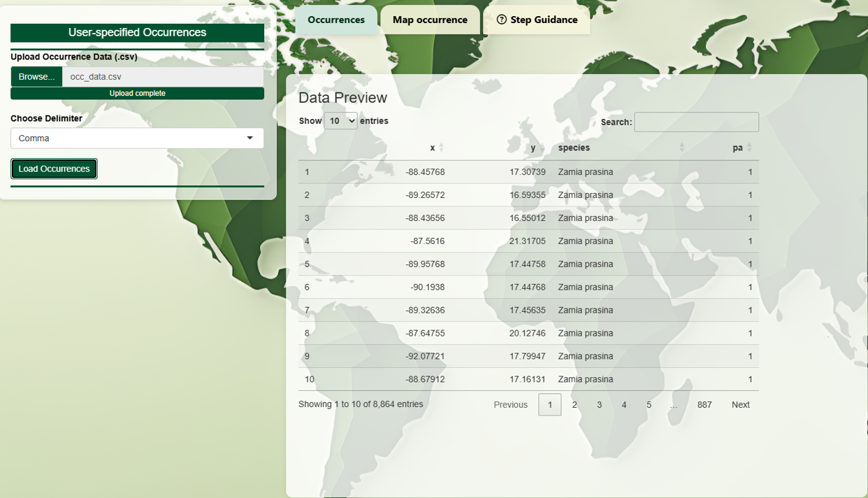
Uploaded occurrence data must follow this structure:
- Longitude (X)
- Latitude (Y)
- Species name (e.g., Zamia prasina)
- Presence/absence (1 = presence, 0 = absence)
The coordinate system must be WGS84 (EPSG:4326) in decimal degrees. Column names are flexible, but the order must be strictly followed. Once your file is successfully loaded, species presence points can be visualized in the Map Occurrence tab to help validate their geographic locations.
Environmental Data
This section guides you through formatting your environmental predictor layers correctly before uploading. The data must be loaded as a SpatRaster object using the terra package in R. It should contain all predictor variables stacked in a single multi-layer raster file (e.g., .tif format).
The raster file must satisfy the following requirements:
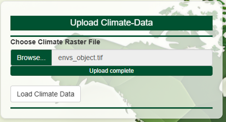
All layers must share the same spatial resolution, extent, and coordinate reference system (CRS). The CRS must be WGS84 (EPSG:4326) in decimal degrees. The file format should be .tif. Avoid .asc or other formats without embedded CRS metadata. Each layer should have a short, interpretable name (e.g., bio1, bio12, slope). After selecting your file, wait until the upload is marked as ‘Upload complete’ before clicking Load Climate Data.
library(terra)
file_path <- 'path/to/your/predictors.tif'
envs <- rast(file_path)
crs(envs) # should return 'EPSG:4326'
After selecting your file, wait until the upload is
marked as ‘Upload complete’ before clicking Load Climate Data.
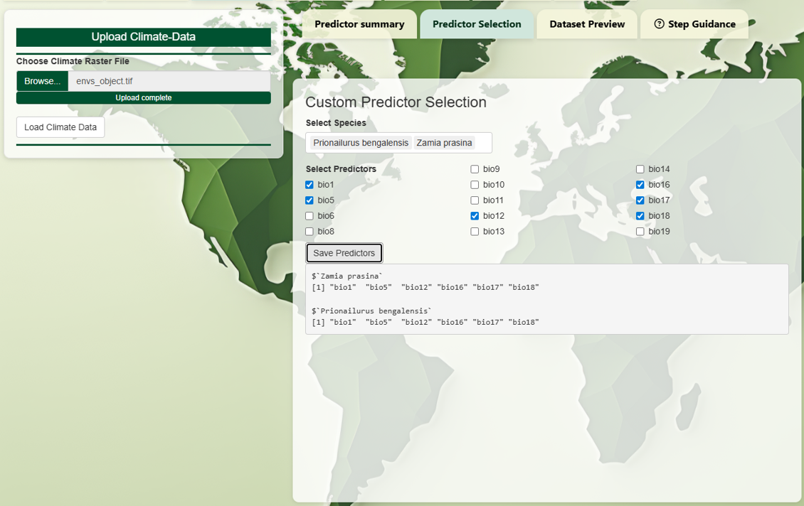
After loading the raster stack, the app summarizes key
statistics (min, max, median, NA count, etc.) for each predictor. Use
this to assess variable ranges, identify missing data, or detect
anomalies. 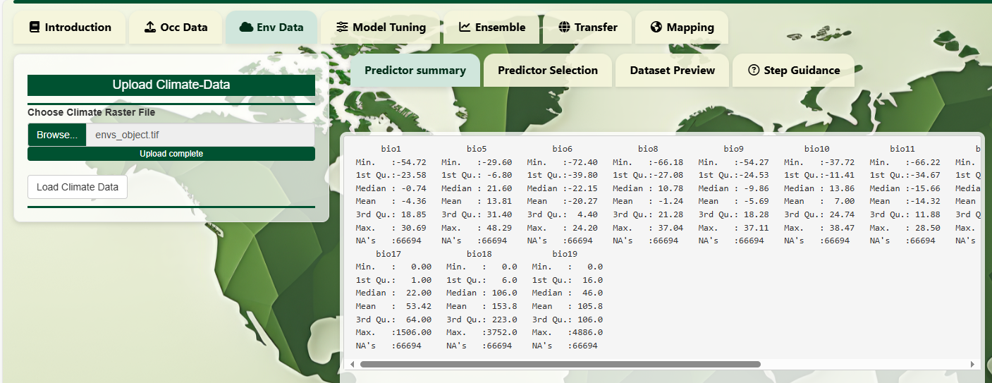
Then, you can select a subset of predictors for each species
individually. This allows more tailored modeling. For example, a
tropical tree and a cold-adapted carnivore may need very different
variables.
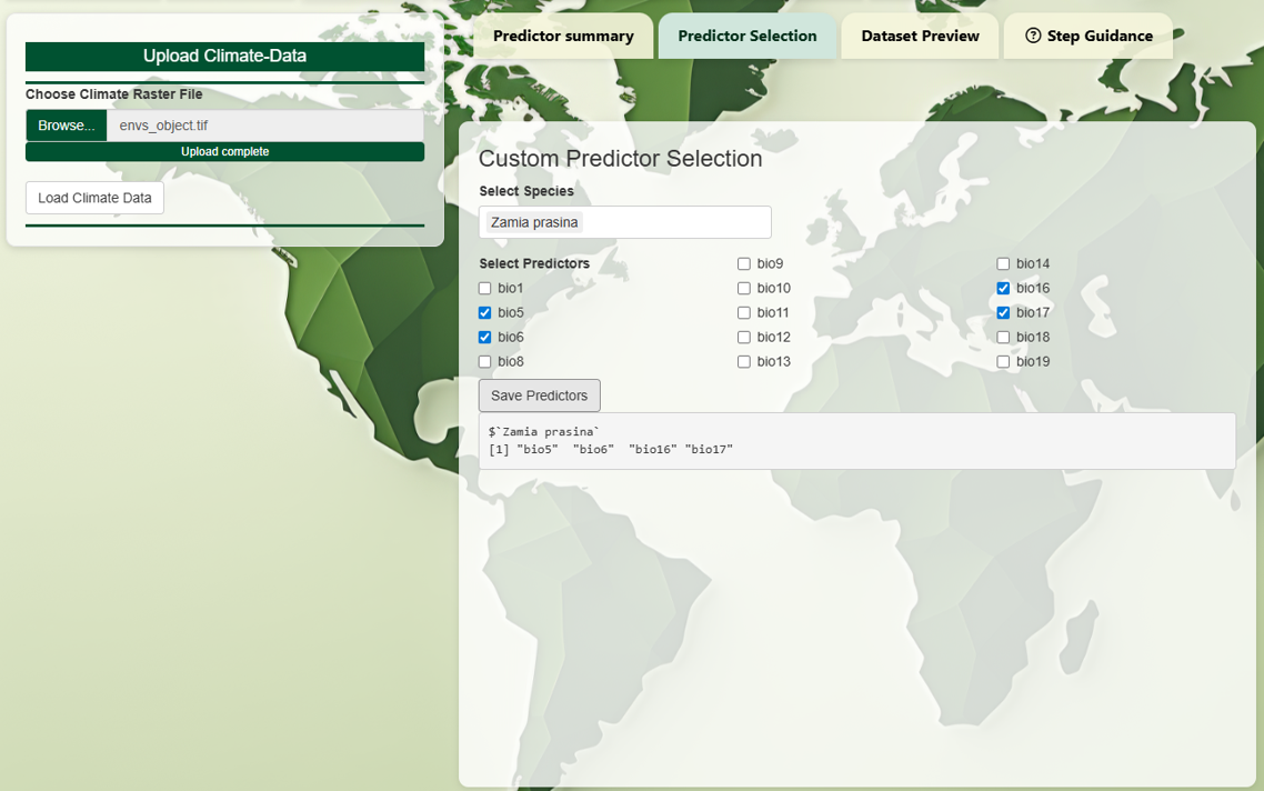
You may choose to assign the same set of predictors to
multiple species.
Model Tuning
How to Tune SDM Models
This section lets you fine-tune Species Distribution Models (SDMs) for each species and algorithm independently, using Bayesian optimization via the tune_bayes() function from the tidymodels ecosystem. You can choose one or more algorithms (e.g., rf, gbm, svm, etc.), and the app will tune each one individually.
Supported models:
- Random Forest (rf)
- XGBoost (gbm)
- Support Vector Machines (SVM)
- Maximum Entropy (Maxent)
- Neural Network (nnet)
- Generalized Additive Model (GAM)
- Generalized Linear Model with quadratic terms to capture non-linearity (GLMsq)
- Multivariate Adaptive Regression Splines (MARS)
- K-Nearest Neighbors (KNN)
Each model is tuned using resampling (e.g., k-fold cross-validation) to find the best hyperparameters. You can customize this process using the following options:
- Initial search size: Number of random models to evaluate before starting Bayesian search.
- Number of iterations: Number of optimization rounds after the initial search.
- Proportion of training data: Fraction of the full dataset used to train models (the remaining used for testing).
- Number of folds: Number of resampling folds used in cross-validation.
- Use parallel: Enable multi-core tuning using the future package.
-
Seed: Set a random seed for reproducibility. Use
0for no seed, or any positive number to ensure reproducible results. - Number of cores: Controls how many processor cores to use when parallelization is enabled.
- Use Weights: Apply optional weighting scheme for presence/absence imbalance.
Specifically, weights are calculated by comparing the number of presence (1) and absence (0) observations:
- If presences are fewer, each presence point is given a higher weight to balance its influence.
- If absences are fewer, the opposite is applied.
The user can activate or deactivate this weighting behavior by
toggling the use_weights parameter.
For example, if you have 100 absences and 20 presences, the weights are:
weight_presences = total_absences / total_presences = 100 / 20 = 5 weight_absences = 1 # default baseline
This means each presence observation is treated as 5 times more important than an absence, helping to correct class imbalance during model fitting.
Once tuning is complete, the following visualizations become
available:
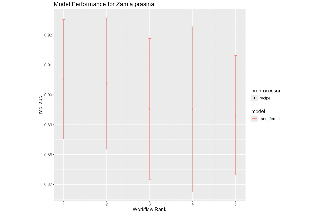
- Tuning Results:
Summary plots showing performance across iterations and models.
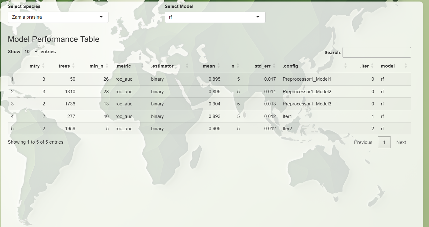
- Tuning Parameters Table: A full
table of all tuned parameter combinations and their metrics.
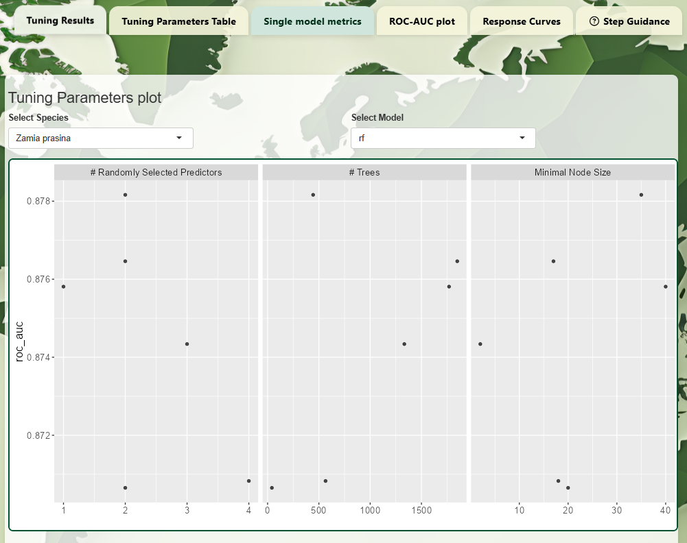
- Single Model Metrics:
Visualization of how individual hyperparameters affect model
performance.
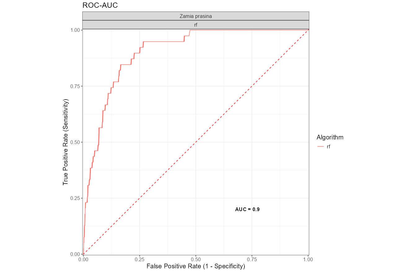
- ROC-AUC Plot: ROC curves based
on the best-tuned model.
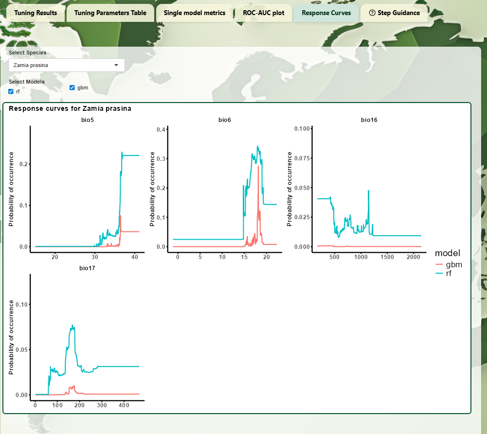
- Response Curves: Partial
dependence plots showing variable influence on predictions.
For more information about the optimization algorithm, see the tune_bayes()
documentation.
Ensemble Modeling
The ensemble module provides a flexible and robust way to combine the
best-performing models into a unified prediction. After model tuning,
multiple candidate models (e.g., rf, gbm,
svm, etc.) are available for each species. Ensemble
modeling helps increase stability and accuracy by leveraging only those
models that meet a specified performance standard.
Selective Inclusion Based on Performance
You can define a performance threshold (e.g., ROC-AUC ≥ 0.85), and the app will:
- Filter all trained models across folds and configurations.
- Retain only the models that exceed the threshold on their individual fold performance.
- Discard poorly performing models, even if they belong to the same algorithm (e.g., only 3 out of 5 Random Forest models might be retained).
This selective process ensures that the ensemble is robust and focused on reliability.
How to Customize the Ensemble
You can interactively control the ensemble process by:
- Adjusting the performance threshold — either globally for all species or individually per species.
- Manually selecting which models or species to include.
- Visualizing ensemble performance through test set ROC-AUC curves.
To assign different thresholds to different species:
- Select a species from the dropdown.
- Adjust the threshold slider.
- Click “Save for one species” to apply the value.
- Repeat for each species.
Alternatively, to apply the same threshold to all species, adjust the slider and click “Apply to All”.
Once thresholds are set and models are selected, click “Run Ensemble” to generate predictions. These predictions will then be used for:
- Model evaluation
- Climate scenario transfer
- Final suitability mapping
Why Ensemble?
The ensemble combines top-performing individual model predictions into a unified output, improving both predictive stability and ecological interpretability.
Model Transfer
Once species distribution models (SDMs) are trained, the Model Transfer module enables you to project them onto new environmental or spatial conditions — such as future climate scenarios or novel geographic regions. This is essential for understanding how species suitability may shift under changing environments.
Input Data:
The .tif file uploaded earlier in the Env
Data section is automatically reused
here.
You do not need to re-upload it unless you wish to
explore a new scenario (e.g., future climate layers or a different
region).
If uploading a new scenario stack:
- Ensure it follows the same layer names, order, and format as the training dataset.
Spatial Cropping Options
You can define the area for model transfer using one of four cropping methods:
- Draw Extent: Manually draw polygons on the map. You can assign unique extents per species.
- Select Countries: Clip predictions using official country boundaries.
- Upload Shapefile: Use your own polygon shapefile (e.g., custom region of interest).
- No Crop: Skip cropping if your raster stack is already trimmed to your target region.
Each cropping method can be:
- Applied globally to all species, or
- Customized individually per species using action buttons (e.g., Apply Drawn Extent to Species).
Species and Model Selection
You can choose to:
- Transfer predictions for one or multiple species.
- Include only selected models (e.g.,
RFandGLM) in the final output.
Ensemble and Filtering
If enabled, ensemble predictions are generated by combining model outputs using a specified method such as:
meanmedian
Even when ensemble mode is active, individual model predictions are always computed and available.
Binarization Options:
You may convert continuous suitability scores into binary (presence/absence) maps using:
Quantile of Minimum Training Presence: e.g., setting a threshold of
0.05excludes the lowest 5% of predicted suitability values at known presence locations. This method allows for more biologically conservative predictions, especially useful for long-lived species like trees.Max Sensitivity + Specificity Threshold: This default method is always included, producing binary predictions optimized for classification accuracy.
Why Transfer Models?
This step helps you explore model behavior in novel contexts — such as future climate, new territories, or ecological restoration zones — providing critical insights for conservation and climate adaptation planning.
Visualizing Model Predictions
This section enables you to visualize the outputs generated by your SDMs, either from individual models or ensemble predictions, across various environmental scenarios.
What You Can Visualize
You can select:
- A species of interest
- A prediction type (e.g., continuous or binary)
- A model or ensemble configuration
The available prediction types include:
-
Proba: Continuous probability values ranging from 0 to 1. -
Max_Sens_Spec_binary: Binary map using the threshold that maximizes sensitivity and specificity. -
Min_training_binary: Binary map using the minimum predicted value at presence training locations. -
Ens_*: Ensemble versions of the above, available if ensemble modeling was applied.
Note: The Max Sensitivity + Specificity threshold is always computed and applied as the default binarization. This binary version is included automatically in visual outputs.
Interpreting the Maps
These visualizations allow you to assess spatial patterns of predicted suitability:
- Under current conditions or future scenarios
- For individual models versus ensemble predictions
By comparing the spatial outputs, you can evaluate how model consensus and thresholding impact the interpretation of habitat suitability across the landscape.